Repeatuntilsuccess Cubic Phase Gate for Universal Continuousvariable Quantum Computation

Note

Click here to download the full example code

CV quantum gate visualizations¶

Author: Brianna Gopaul

In a conventional quantum circuit, qubits represented by wires are operated on by quantum gates which collectively perform computations. Similarily, continuous variable quantum computing uses qumodes that represent bundles of interacting photons. To perform computations on qumodes, we leverage Gaussian and non-Gaussian gates.

Gaussian and non-Gaussian gates can be described within the phase space. This space is shown by the position and momentum axes.

Gaussian gates such as the squeezing and rotation gate act linearly on modes. These gates can only reach positive quasi-probability distributions and can be classically simulated. On the other hand, non-Gaussian gates such as the Kerr gate and Cubic Phase gate act nonlinearly. This property allows them to be in negative quasi-probability distributions and not be classically simulated.

In this notebook, we'll learn about various single mode Gaussian and non-Gaussian gates and apply them to a state using Strawberry Fields.

                            import              strawberryfields              as              sf              from              strawberryfields.ops              import              *              import              numpy              as              np              import              matplotlib.pyplot              as              plt              from              mpl_toolkits.mplot3d              import              Axes3D            

Vacuum State¶

The vacuum state is the lowest energy Gaussian state. It has no displacement or squeezing in phase space.

Here we learn how to create the vacuum state on a quantum circuit with one qumode.

We initialize the Strawberry Fields program. q represents a qumode and below we start with one qumode for our circuit.

We declare our quantum circuit using the engine. We can prepare the Vacuum state on one qumode using | .

It should be noted that the default state in strawberry fields is the vacuum state. The above gate is listed to show the operation.

In Strawberry Fields, there are three main backends that can be used to perform computations. The backend selected will depend on the task you want to perform. Above, we've used the Gaussian backend to run our vacuum state circuit. We can also alternatively use the Fock backend to run the circuit. The third backend is the tensorflow backend 'tf'. It leverages tensorflow to create quantum machine learning models.

Using matplotlib, we then plot the Wigner function of the vacuum state, which is a Gaussian distribution. The Wigner function quasi-probability illustrates negative and positive regions in phase space. We'll notice below that Gaussian states such as the vacuum and squeezed state are in positive regions of phase space while non-Gaussian states can reach negative regions of the phase space. The y-axis on this plot can describe the \(\hat {p}\) quadrature or momentum operator and the x-axis describes the \(\hat{x}\) quadrature or position operator of the state.

                                fig                =                plt                .                figure                ()                X                =                np                .                linspace                (                -                5                ,                5                ,                100                )                P                =                np                .                linspace                (                -                5                ,                5                ,                100                )                Z                =                state                .                wigner                (                0                ,                X                ,                P                )                X                ,                P                =                np                .                meshgrid                (                X                ,                P                )                ax                =                fig                .                add_subplot                (                111                ,                projection                =                "3d"                )                ax                .                plot_surface                (                X                ,                P                ,                Z                ,                cmap                =                "RdYlGn"                ,                lw                =                0.5                ,                rstride                =                1                ,                cstride                =                1                )                fig                .                set_size_inches                (                4.8                ,                5                )                ax                .                set_axis_off                ()              

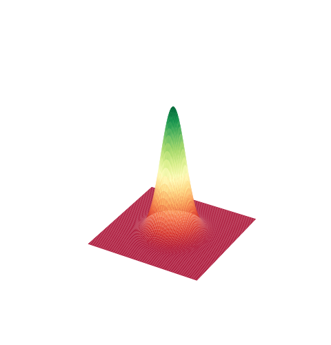
We can make a couple of observations from the Gaussian distribution above. We notice that it has positive quasi-probability everywhere. Later on, we'll have a look at non-Gaussian gates that have regions of negative quasi-probability. The vacuum state is also centered at 0 on both the position axis \(\hat {x}\) and momentum axis \(\hat {p}\).

Squeezing Gate¶

The squeezing gate can also be thought of as a transformation on the position and momentum axes. The squeezing gate scales \(x\) to \(e^{ - r}\hat{x} _\phi\) and scales \(p\) with \(e^{r}\hat{p} _\phi\). In the Wigner function, we can see the probability distribution being lengthened on the momentum axis and being pinched on the position axis. As the squeezing gate is a Gaussian gate, there are no regions of negative quasi-probabilty.

                                prog                =                sf                .                Program                (                1                )                with                prog                .                context                as                q                :                S                =                Sgate                (                1                )                S                |                q                [                0                ]                state                =                eng                .                run                (                prog                )                .                state                fig                =                plt                .                figure                ()                X                =                np                .                linspace                (                -                5                ,                5                ,                100                )                P                =                np                .                linspace                (                -                5                ,                5                ,                100                )                Z                =                state                .                wigner                (                0                ,                X                ,                P                )                X                ,                P                =                np                .                meshgrid                (                X                ,                P                )                ax                =                fig                .                add_subplot                (                111                ,                projection                =                "3d"                )                fig                .                set_size_inches                (                4.8                ,                5                )                ax                .                plot_surface                (                X                ,                P                ,                Z                ,                cmap                =                "RdYlGn"                ,                lw                =                0.5                ,                rstride                =                1                ,                cstride                =                1                )                ax                .                set_axis_off                ()              

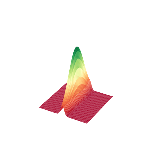
The below animation shows the squeezing gate acting on the vacuum state with increasing strengths of parameters.

Rotation Gate¶

The rotation gate shifts the \(\hat{x}\) quadrature to \(\hat{x}\) \(\cos \phi\) - \(\hat{p}\sin\) \(\phi\) and \(\hat{p}\) to \(\hat{p}\) \(\cos \phi\) + \(\hat{x}\sin\) \(\phi\). In other words, the gate simply rotates the phase space.

                                prog                =                sf                .                Program                (                1                )                with                prog                .                context                as                q                :                Dgate                (                1                )                |                q                [                0                ]                Rgate                (                np                .                pi                /                2                )                |                q                [                0                ]                eng                .                reset                ()                state                =                eng                .                run                (                prog                )                .                state                fig                =                plt                .                figure                ()                X                =                np                .                linspace                (                -                5                ,                5                ,                100                )                P                =                np                .                linspace                (                -                5                ,                5                ,                100                )                Z                =                state                .                wigner                (                0                ,                X                ,                P                )                X                ,                P                =                np                .                meshgrid                (                X                ,                P                )                ax                =                fig                .                add_subplot                (                111                ,                projection                =                "3d"                )                ax                .                plot_surface                (                X                ,                P                ,                Z                ,                cmap                =                "RdYlGn"                ,                lw                =                0.5                ,                rstride                =                1                ,                cstride                =                1                )                fig                .                set_size_inches                (                4.8                ,                5                )                ax                .                set_axis_off                ()              

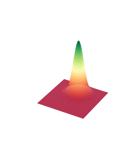
Above we apply the rotation gate to a coherent state. When compared to the squeezed state in the previous example, the rotation gate simply makes a rotation.

Similarily, the rotation gate is applied with an increasing parameter in the below animation.

Displacement Gate¶

The displacement gate has a specified complex value \(\alpha\). It shifts \(\hat{x}\) by a value porportional to \(Re(\alpha)\) and the \(\hat {p}\) by a value \(Im({\alpha})\).

                                prog                =                sf                .                Program                (                1                )                with                prog                .                context                as                q                :                Dgate                (                0.55                )                |                q                [                0                ]                eng                .                reset                ()                state                =                eng                .                run                (                prog                )                .                state                fig                =                plt                .                figure                ()                X                =                np                .                linspace                (                -                5                ,                5                ,                100                )                P                =                np                .                linspace                (                -                5                ,                5                ,                100                )                Z                =                state                .                wigner                (                0                ,                X                ,                P                )                X                ,                P                =                np                .                meshgrid                (                X                ,                P                )                ax                =                fig                .                add_subplot                (                111                ,                projection                =                "3d"                )                ax                .                plot_surface                (                X                ,                P                ,                Z                ,                cmap                =                "RdYlGn"                ,                lw                =                0.5                ,                rstride                =                1                ,                cstride                =                1                )                fig                .                set_size_inches                (                4.8                ,                5                )                ax                .                set_axis_off                ()              

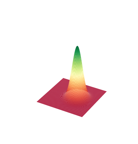
As \(\alpha\) increases in value, the state is displaced more to the right.

Cubic Phase Gate¶

The cubic phase gate shifts \(\hat{p}\) by \(\gamma\hat{x}^2\) where \(\gamma\) is a definable parameter but does not transform \(\hat{x}\) in the phase space. Below, we decide to set \(\gamma=2\).

When running a circuit that contains any non-Gaussian gates, we use the Fock backend. Depending on the backend used, different arguments will have to be called. In this example, we define 'cutoff_dim' which tells Strawberry Fields where to limit the Fock space.

                                prog                =                sf                .                Program                (                1                )                with                prog                .                context                as                q                :                gamma                =                2                Vgate                (                gamma                )                |                q                [                0                ]                #We use the fock backend and define the argument cutoff_dim                eng                =                sf                .                Engine                (                'fock'                ,                backend_options                =                {                "cutoff_dim"                :                10                })                state                =                eng                .                run                (                prog                )                .                state                fig                =                plt                .                figure                ()                X                =                np                .                linspace                (                -                5                ,                5                ,                100                )                P                =                np                .                linspace                (                -                5                ,                5                ,                100                )                Z                =                state                .                wigner                (                0                ,                X                ,                P                )                X                ,                P                =                np                .                meshgrid                (                X                ,                P                )                ax                =                fig                .                add_subplot                (                111                ,                projection                =                "3d"                )                ax                .                plot_surface                (                X                ,                P                ,                Z                ,                cmap                =                "RdYlGn"                ,                lw                =                0.5                ,                rstride                =                1                ,                cstride                =                1                )                fig                .                set_size_inches                (                4.8                ,                5                )                ax                .                set_axis_off                ()              

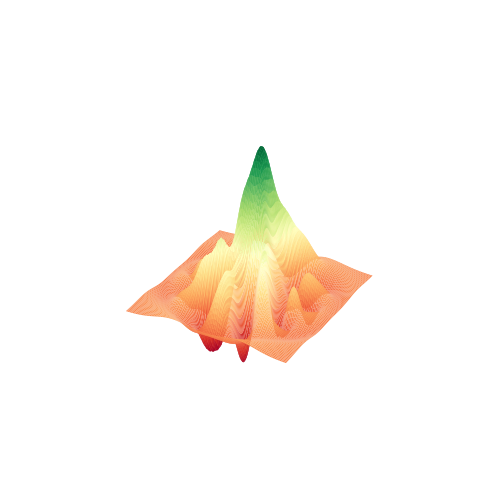
Here we can see that the vacuum state has been shifted to a state where it reaches negative quasi-probability distributions.

Kerr Gate¶

Before we understand how the Kerr gate operates, we should first take another look at the rotation gate. In the Fock basis, the rotation gate acts with \(e^{ i\phi \hat{n}}\). In comparison, the Kerr gates transforms with \(e^{ i\phi k \hat{n}^2}\). The \(^2\) value is what makes this state non-Gaussian and thus transforms the shape of the state significantly.

                                prog                =                sf                .                Program                (                1                )                with                prog                .                context                as                q                :                kappa                =                1                Dgate                (                1                )                |                q                [                0                ]                Kgate                (                kappa                )                |                q                [                0                ]                eng                .                reset                ()                state                =                eng                .                run                (                prog                )                .                state                fig                =                plt                .                figure                ()                X                =                np                .                linspace                (                -                5                ,                5                ,                100                )                P                =                np                .                linspace                (                -                5                ,                5                ,                100                )                Z                =                state                .                wigner                (                0                ,                X                ,                P                )                X                ,                P                =                np                .                meshgrid                (                X                ,                P                )                ax                =                fig                .                add_subplot                (                111                ,                projection                =                "3d"                )                ax                .                plot_surface                (                X                ,                P                ,                Z                ,                cmap                =                "RdYlGn"                ,                lw                =                0.5                ,                rstride                =                1                ,                cstride                =                1                )                fig                .                set_size_inches                (                4.8                ,                5                )                ax                .                set_axis_off                ()              

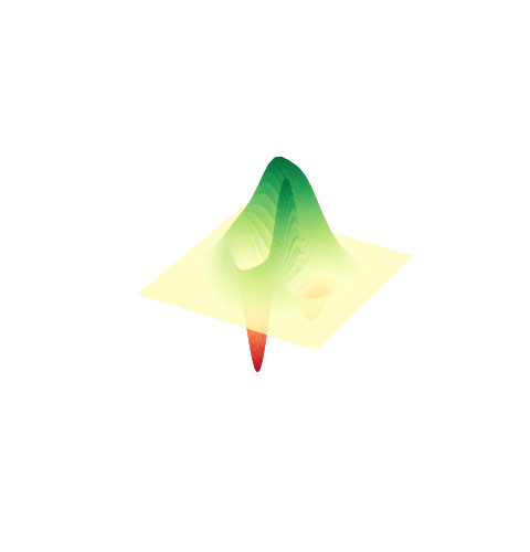
In the below Wigner function, the state is initially in a coherent state.

We can see it's coherent structure morphing after the Kerr gate is applied at different strengths.

For more information about CV gates, see the CV gates section in the Strawberry Fields documentation.

Total running time of the script: ( 0 minutes 4.172 seconds)

Gallery generated by Sphinx-Gallery

demos/run_gate_visualization

andersondeston.blogspot.com

Source: https://strawberryfields.ai/photonics/demos/run_gate_visualization.html

Share this post